Tetrahedra FE pipeline - embedded human tooth; heterogeneous materials
Created on: 30.04.2022
Last update: 30.07.2022
By: Gianluca Iori, 2023
Data source: the dataset used in this example is courtesy of Prof. Rachel Sarig, Sackler Faculty of Medicine, Tel Aviv University.
Code license: MIT
Narrative license: CC-BY-NC-SA
Aims
The example implements the following ciclope pipeline:
Load and inspect microCT volume data of a human tooth
Image preprocessing
Segment different tissue types (enamel, dentin)
Map different scalars to the 3D image to represent different tissues
Add embedding material (dental cement) with given Grey Value
Add end-caps (steel) with given Grey Value
Generate 3D Unstructured Grid mesh of tetrahedra
Generate tetrahedra-FE model for simulation in CalculX or Abaqus from 3D Unstructured Grid mesh
Linear, static analysis definition: displacement-driven uniaxial compression test
Local material mapping (assign one material card to each dataset grey value)
Launch simulation in Calculix. For info on the solver visit the Calculix homepage
Convert Calculix output to .VTK for visualization in Paraview
Automatic plot of displacement field mid-planes through the model
Type python ciclope.py -h to display the ciclope help with a full list of available command line arguments.
Configuration and imports
import sys
sys.path.append('./../../')
import numpy as np
import matplotlib
import matplotlib.pyplot as plt

import mcubes
from scipy import ndimage, misc
from skimage.filters import threshold_otsu, threshold_multiotsu, gaussian
from skimage import morphology
import skimage.io as skio

from ciclope.utils.recon_utils import plot_midplanes, bbox
from ciclope.utils.preprocess import fill_voids, embed, add_cap
from ciclope import tetraFE

matplotlib.rcParams['figure.dpi'] = 200

font = {'weight' : 'normal',
        'size'   : 8}

plt.rc('font', **font)
Load input data
input_file = './../../test_data/tooth/Tooth_3_scaled_2.tif' # scale factor: 0.4
data_3D = skio.imread(input_file, plugin="tifffile")
vs = np.ones(3)*16.5e-3/0.4 # [mm]
Inspect the dataset
plot_midplanes(data_3D)

Inspect the dataset with itkwidgets
# import itk
# from itkwidgets import view
# viewer = view(data_3D, ui_collapsed=True)
# viewer.interpolation = False
# # launch itk viewer
# viewer
Pre-processing
Thresholding
Find multiple Otsu’s thresholds
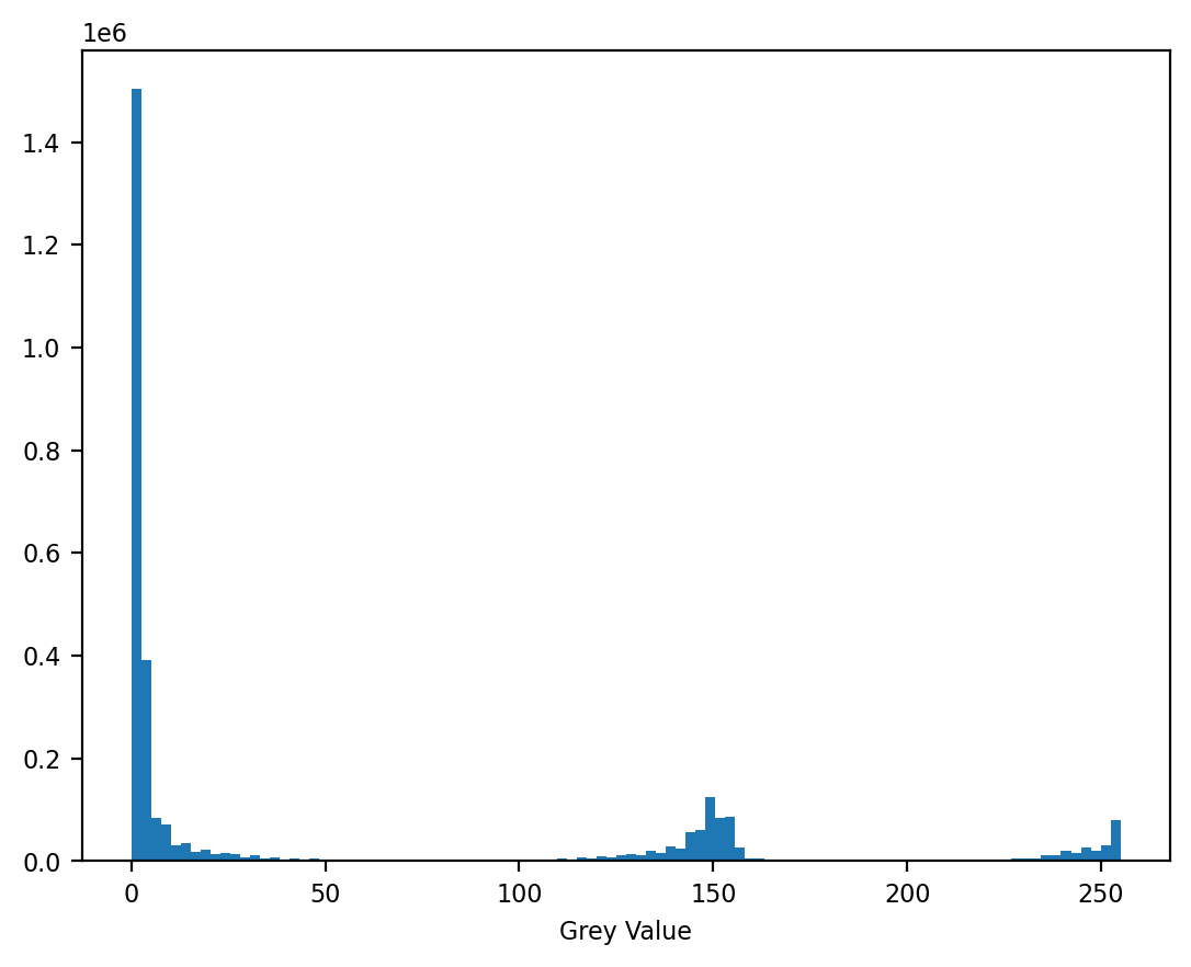
Ts = threshold_multiotsu(data_3D)
print("Thresholds: {}".format(Ts))
Thresholds: [ 73 193]
Plot the dataset histogram
# plot the input image histogram
fig2, ax2 = plt.subplots()
plt.hist(data_3D.ravel(), bins=100)
plt.xlabel('Grey Value')
plt.show()
plt.style.use('seaborn')
/tmp/ipykernel_28098/656133569.py:6: MatplotlibDeprecationWarning: The seaborn styles shipped by Matplotlib are deprecated since 3.6, as they no longer correspond to the styles shipped by seaborn. However, they will remain available as 'seaborn-v0_8-<style>'. Alternatively, directly use the seaborn API instead.
  plt.style.use('seaborn')
Apply the thresholds
Separate the whole tooth volume, dentin and enamel areas
BW_tooth = data_3D >= Ts[0]
BW_dentin = (data_3D <= Ts[1]) & (data_3D >= Ts[0])
BW_enamel = data_3D > Ts[1]
Morphological cleaning of the masks
Opply morphological open and fill holes within the dentin mask
BW_dentin = ndimage.binary_fill_holes(ndimage.binary_opening(BW_dentin, morphology.ball(3)))
BW_tooth = ndimage.binary_fill_holes(ndimage.binary_opening(BW_tooth, morphology.ball(3)))
plt.style.use('default')
plot_midplanes(BW_tooth)
Create color image with different materials
Our goal is to create a 3D image of the tooth + embedding and assign the following scalars to the different materials:
dentin
enamel
cement embedding
steel caps
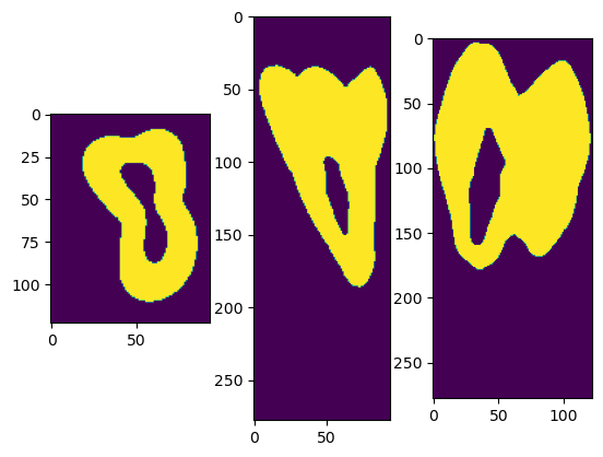
We start by creating an image of the tooth where dentin and enamel have different Grey Values (1 and 2, respectively)
data_for_meshing = fill_voids(BW_dentin*1 + BW_enamel*2, 1, False)
plot_midplanes(data_for_meshing)

Embed tooth from top and bottom
Add embedding material (cement) from the bottom and top along the image Z-axis. The method ciclope.utils.preprocess.embed allows to embed a 3D image from a chosen direction and to specify the Grey Value of the embedding material. For a full list of embedding parameters see the method help typing:
help(embed)
Help on function embed in module ciclope.utils.preprocess:

embed(I, embed_depth, embed_dir, embed_val=None, pad=0, makecopy=False)
    Add embedding to 3D image.
    Direction and depth of the embedded region should be given. Zeroes in the input image is considered to be background.

    Parameters
    ----------
    I
        3D data. Zeroes as background.
    embed_depth : int
        Embedding depth in pixels.
    embed_dir : str
        Embedding direction. Can be "-x", "+x", "-y", "+y", "-z", or "+z".
    embed_val : float
        Embedding grey value.
    pad = int
        Padding around bounding box of embedded area.
    makecopy : bool
        Make copy of the input image.

    Returns
    ----------
    I
        Embedded image. Same size as the input one.
    BW_embedding
        BW mask of the embedding area.
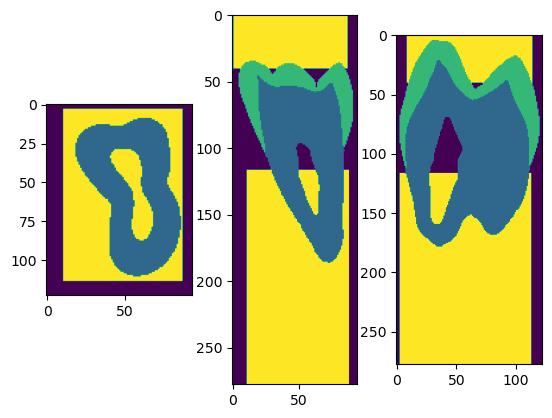
Embed from the bottom along the X-axis over 140 image voxels. Assign Grey Value = 3 to the embedding material:
data_for_meshing_embedded, BW_embedding_bottom = embed(data_for_meshing, 140, "-z", embed_val=3, pad=2, makecopy=True)
Embed from the top along the X-axis over 40 image voxels. Assign Grey Value = 3 to the embedding material:
data_for_meshing_embedded, BW_embedding_top = embed(data_for_meshing_embedded, 40, "+z", embed_val=3, pad=2)
plot_midplanes(data_for_meshing_embedded)
Add steel caps
The method ciclope.utils.preprocess.add_cap allows to add caps to a 3D image from a chosen direction, with a given thickness and Grey Value.
To see the method help type help(ciclope.utils.preprocess.add_cap
Add 5-voxels-thick caps with GV=4:
data_for_meshing_embedded = add_cap(data_for_meshing_embedded, cap_thickness=5, cap_val=4)
plot_midplanes(data_for_meshing_embedded)

Create tetrahedra mesh
Volume meshing using CGAL through pygalmesh
filename_mesh_out = './../../test_data/tooth/results/Tooth_3_scaled_2.vtk'
Reduce the mesh_size_factor (keeping it small for fast execute)
mesh_size_factor = 5 # 1.2
mesh = tetraFE.cgal_mesh(data_for_meshing_embedded, vs, 'tetra', mesh_size_factor * min(vs), 3* mesh_size_factor * min(vs))

Write Abaqus input FE files
Generate tetrahedra-FE model with multiple material properties
The method ciclope.core.tetraFE.mesh2tetrafe assumes that the material property definition is contained in the FE analysis .INP template file.
input_template = "./../../input_templates/tmp_example03_comp_static_tooth.inp"
Inspect input template file:
The first section of the input template contains material definitions for the four materials of the model
The next section defines a static linear-step analysis with the following boundary conditions:
Displacement along Z = 0 for all nodes on the model top surface (NODES_Z1)
Displacement completely fixed (X=0, Y=0, Z=0) for the nodes at the (0,0,0) corner. This is to avoid free-body motion
0.25 mm displacement imposed along Z on all nodes on the bottom surface (NODES_Z0)
!cat {input_template} # on linux
** User material property definition:
** ---------------------------------------------------
** DENTIN - https://www.ncbi.nlm.nih.gov/pmc/articles/PMC3924884/
** ---------------------------------------------------
*SOLID SECTION, ELSET=SET1, MATERIAL=DENTIN
1.
*MATERIAL,NAME=DENTIN
*ELASTIC
1653.7, 0.3
** ---------------------------------------------------
** ENAMEL
** ---------------------------------------------------
*SOLID SECTION, ELSET=SET2, MATERIAL=ENAMEL
1.
*MATERIAL,NAME=ENAMEL
*ELASTIC
1338.2, 0.3
** ---------------------------------------------------
** CEMENT H poly - https://brieflands.com/articles/zjrms-94390.html
** ---------------------------------------------------
*SOLID SECTION, ELSET=SET3, MATERIAL=CEMENT
1.
*MATERIAL,NAME=CEMENT
*ELASTIC
2200., 0.3
** ---------------------------------------------------
** STEEL
** ---------------------------------------------------
*SOLID SECTION, ELSET=SET4, MATERIAL=STEEL
1.
*MATERIAL,NAME=STEEL
*ELASTIC
210000., 0.333
** ---------------------------------------------------
** Analysis definition. The Step module defines the analysis steps and associated output requests.
** More info at:
** https://abaqus-docs.mit.edu/2017/English/SIMACAECAERefMap/simacae-m-Sim-sb.htm#simacae-m-Sim-sb
** Impose vertical displacement on NODES_Z0; NODES_Z1 completely constrained.
** ---------------------------------------------------
*STEP
*STATIC
*BOUNDARY
NODES_Z1, 3, 3, 0.0
*BOUNDARY
NODES_X0Y0Z0, 1, 3, 0.0
*BOUNDARY
NODES_Z0, 3, 3, 0.5
** ---------------------------------------------------
** Output request:
*NODE FILE, OUTPUT=2D
U
*NODE PRINT, TOTALS=ONLY, NSET=NODES_Z0
RF
*EL FILE, OUTPUT=2D
S, E
*END STEP
filename_out = './../test_data/tooth/results/Tooth_3_scaled_2.inp'
Generate CalculiX FE input file
tetraFE.mesh2tetrafe(mesh, input_template, filename_out, keywords=['NSET', 'ELSET'])
Solve FE model in calculix
The following section assumes that you have the Calculix solver installed and accessible with the command ccx_2.17 or for multithread option ccx_2.17_MT.
The multithread option in CalculiX is activated by defining the number of threads (default=1) used for the calculation.
This is done by setting the env variable OMP_NUM_THREADS with:
export OMP_NUM_THREADS=8
!export OMP_NUM_THREADS=8; ccx_2.17_MT "./../../test_data/tooth/results/Tooth_3_scaled_2"
************************************************************

CalculiX Version 2.17, Copyright(C) 1998-2020 Guido Dhondt
CalculiX comes with ABSOLUTELY NO WARRANTY. This is free
software, and you are welcome to redistribute it under
certain conditions, see gpl.htm

************************************************************

You are using an executable made on Sun 10 Jan 2021 11:34:19 AM CET

  The numbers below are estimated upper bounds

  number of:

   nodes:        43539
   elements:       239463
   one-dimensional elements:            0
   two-dimensional elements:            0
   integration points per element:            1
   degrees of freedom per node:            3
   layers per element:            1

   distributed facial loads:            0
   distributed volumetric loads:            0
   concentrated loads:            0
   single point constraints:         1668
   multiple point constraints:            1
   terms in all multiple point constraints:            1
   tie constraints:            0
   dependent nodes tied by cyclic constraints:            0
   dependent nodes in pre-tension constraints:            0

   sets:           19
   terms in all sets:       729582

   materials:            4
   constants per material and temperature:            2
   temperature points per material:            1
   plastic data points per material:            0

   orientations:            0
   amplitudes:            3
   data points in all amplitudes:            3
   print requests:            1
   transformations:            0
   property cards:            0


 STEP            1

 Static analysis was selected

 Decascading the MPC's

 Determining the structure of the matrix:
 number of equations
 128951
 number of nonzero lower triangular matrix elements
 2719997

 Using up to 8 cpu(s) for the stress calculation.

 Using up to 8 cpu(s) for the symmetric stiffness/mass contributions.

 Factoring the system of equations using the symmetric spooles solver
 Using up to 8 cpu(s) for spooles.

 Using up to 8 cpu(s) for the stress calculation.


 Job finished

________________________________________

Total CalculiX Time: 20.641087
________________________________________
Post-processing
Convert Calculix output to Paraview
The following sections assume that you have ccx2paraview and Paraview installed and working.
For more info visit:
import os
import ccx2paraview
filename_out_base, ext_out = os.path.splitext(filename_out)
ccx2paraview.Converter(filename_out_base + '.frd', ['vtk']).run()
Visualize results in Paraview
Max. Z-displacement: 0.5 mm
Max. Von Mises stress: 150 MPa
!paraview {filename_out_base + '.vtk'}

Post-process FE analysis results
Display the CalculiX FE output .DAT file containing the total reaction force:
filename_dat = filename_out_base + '.dat'
!cat {filename_dat}
 total force (fx,fy,fz) for set NODES_Z0 and time  0.1000000E+01

        5.069543E-10  4.957852E-10  2.068063E+03
The total reaction force along Z reaches 2068 N