Voxel microFE pipeline - trabecular bone
From micro-CT image to voxel-uFE model solution in Calculix
Created on: 23.05.2021
Last update: 15.01.2023
By: Gianluca Iori, Martino Pani, Gianluigi Crimi, Enrico Schileo, Fulvia Taddei, Giulia Fraterrigo, 2023
Data source: the dataset used in this example is part of the public collection of the Living Human Digital Library (LHDL) Project, a project financed by the European Commission (project number: FP6-IST 026932). Human tissues in the LHDL project were collected according to the body donation program of Universitè Libre de Bruxelles (ULB), partner of the project. For info on the dataset see here.
Code license: MIT
Narrative license: CC-BY-NC-SA
Aims
 The example implements the following ciclope pipeline:
Load and inspect microCT volume data
Image pre-processing
Apply Gaussian smooth (optional)
Resample the dataset (optional)
Segment bone tissue
Remove unconnected clusters of voxels
Mesh generation
Generate 3D Unstructured Grid voxel of hexahedra (voxels)
Generate voxel-FE model for simulation in CalculX or Abaqus from 3D voxel mesh
Linear, static analysis definition: uniaxial compression test
Launch simulation in Calculix. For info on the solver visit the Calculix homepage
Convert Calculix output to .VTK for visualization in Paraview
Calculate apparent elastic modulus from reaction forces
Notes on ciclope
All mesh exports are performed with the meshio module.
ciclope handles the definition of material properties and FE analysis parameters (e.g. boundary conditions, simulation steps..) through separate template files. The folders material_properties and input_templates contain a library of template files that can be used to generate FE simulations.
Command line execution of this example
The pipeline described in this notebook can be executed from the command line using the ciclope command:
ciclope test_data/LHDL/3155_D_4_bc/cropped/3155_D_4_bc_0000.tif test_data/LHDL/3155_D_4_bc/results/3155_D_4_bc_voxelFE.inp -vs 0.0195 0.0195 0.0195 -r 2 -t 63 --smooth 1 --voxelfe --template input_templates/tmp_example01_comp_static_bone.inp
Type python ciclope.py -h to display the ciclope help with a full list of available command line arguments.
Configuration and imports
import sys
sys.path.append('./../../')
import os
import numpy as np
import dxchange
import matplotlib
import matplotlib.pyplot as plt

import mcubes
from scipy import ndimage, misc
from skimage.filters import threshold_otsu, gaussian
from skimage import measure, morphology

from ciclope.utils.recon_utils import read_tiff_stack, plot_midplanes
from ciclope.utils.preprocess import remove_unconnected
import ciclope
Uncomment and run the following cell for visualizations using itkwidgets
# import itk
# from itkwidgets import view
# import vtk
ccx2paraview is needed for the postprocessing of results
import ccx2paraview
matplotlib.rcParams['figure.dpi'] = 300

font = {'weight' : 'normal',
        'size'   : 6}

plt.rc('font', **font)
Load input data
input_file = './../../test_data/LHDL/3155_D_4_bc/cropped/3155_D_4_bc_0000.tif'
Input data description
Scan parameters |
|
|---|---|
Lab |
LTM@IOR Bologna |
Sample |
Human trabecular bone |
Voxel size |
19.5 micron |
Preliminary operations |
Cropped to 200x200x200 (4mm side) |
Read the input data and define an array of the voxelsize
data_3D = read_tiff_stack(input_file)
vs = np.ones(3)*19.5e-3 # [mm]
type(data_3D)
numpy.ndarray
Inspect the dataset
plot_midplanes(data_3D)
plt.show()

Inspect the dataset with itkwidgets
# viewer = view(data_3D, ui_collapsed=True)
# viewer.interpolation = False
Launch itk viewer
# viewer
Pre-processing
Gaussian smooth
data_3D = gaussian(data_3D, sigma=1, preserve_range=True)
Resize (downsample) with factor 2
resampling = 2

# resize the 3D data using spline interpolation of order 2
data_3D = ndimage.zoom(data_3D, 1/resampling, output=None, order=2)

# correct voxelsize
vs = vs * resampling
# Inspect again the dataset
plot_midplanes(data_3D)
plt.show()

Thresholding
Use Otsu’s method
T = threshold_otsu(data_3D)
print("Threshold: {}".format(T))
Threshold: 80.72472439570987
# plot the input image histogram
fig2, ax2 = plt.subplots()
plt.hist(data_3D.ravel(), bins=40)
plt.show()

Apply single global threshold obtained from comparison with histology
# BW = data_3D > T
BW = data_3D > 63 # from comparison with histology
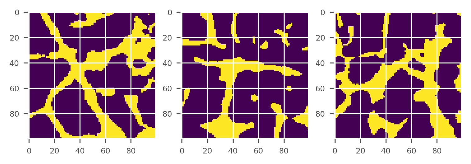
Have a look at the binarized dataset
plot_midplanes(BW)
plt.show()
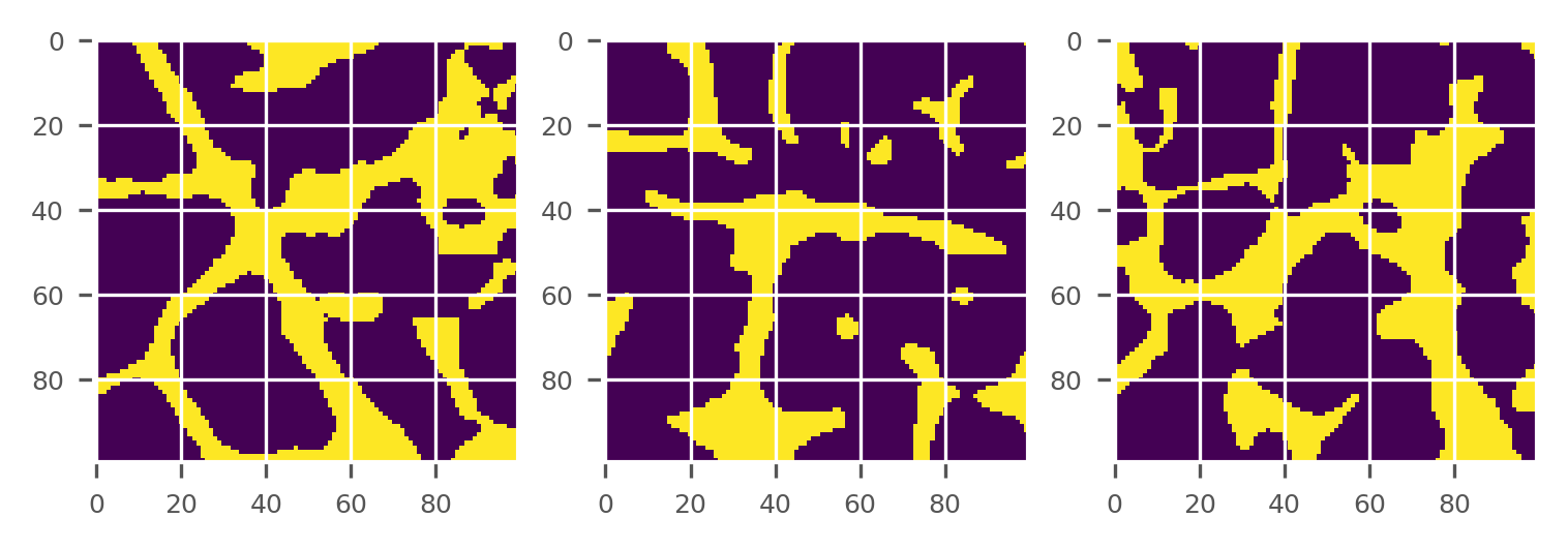
Morphological close of binary image (optional)
BW = morphology.closing(BW, morphology.ball(3))
plot_midplanes(BW)
plt.show()
Detect largest isolated cluster of voxels
The procedure is described by the following 3 steps:
Label the BW 3D image
# [labels, n_labels] = measure.label(BW, None, True, 1) # 1 connectivity hop
Count the occurrences of each label
# occurrences = np.bincount(labels.reshape(labels.size))
Find the largest unconnected label
# largest_label_id = occurrences[1:].argmax()+1
# L = labels == largest_label_id
You can do the same using the function remove_unconnected contained in ciclope.utils.preprocess
L = remove_unconnected(BW)
Inspect dataset
plot_midplanes(L)
plt.show()
Generate Unstructured Grid Mesh of hexahedra from volume data
mesh = ciclope.core.voxelFE.vol2ugrid(L, vs, verbose=True)
INFO:root:Calculating cell array
INFO:root:Detecting node coordinates and boundary nodes
INFO:root:Generated the following mesh with 1030301 nodes and 247062 elements:
INFO:root:<meshio mesh object>
  Number of points: 1030301
  Number of cells:
    hexahedron: 247062
  Point sets: NODES_Y1, NODES_Y0, NODES_X0, NODES_X1, NODES_Z1, NODES_Z0, NODES_X0Y0Z0, NODES_X0Y0Z1
  Cell sets: CELLS_Y1, CELLS_Y0, CELLS_X0, CELLS_X1, CELLS_Z1, CELLS_Z0
  Cell data: GV
Write the mesh using meshio:
Support for binary data type is not included. We cast GV cell_data to uint8
mesh.cell_data['GV'] = mesh.cell_data['GV'][0].astype('uint8')
print(mesh)
<meshio mesh object>
  Number of points: 1030301
  Number of cells:
    hexahedron: 247062
  Point sets: NODES_Y1, NODES_Y0, NODES_X0, NODES_X1, NODES_Z1, NODES_Z0, NODES_X0Y0Z0, NODES_X0Y0Z1
  Cell sets: CELLS_Y1, CELLS_Y0, CELLS_X0, CELLS_X1, CELLS_Z1, CELLS_Z0
  Cell data: GV
filename_mesh_out = './../../test_data/LHDL/3155_D_4_bc/results/3155_D_4_bc_voxelmesh.vtk'
mesh.write(filename_mesh_out)
Visualize the mesh with itkwidgtes
# reader = vtk.vtkUnstructuredGridReader()
# reader.SetFileName(filename_mesh_out)
# reader.Update()
# grid = reader.GetOutput()
# view(geometries=grid)

Write CalculiX input FE files
Generate voxel-FE model with constant material properties
If a binary ndarray is given as input, the script vol2voxelfe will assume that the material property definition is contained in the FE analysis .INP template file.
https://classes.engineering.wustl.edu/2009/spring/mase5513/abaqus/docs/v6.6/books/usb/default.htm?startat=pt05ch17s02abm02.html
filename_out = './../../test_data/LHDL/3155_D_4_bc/results/3155_D_4_bc_voxelFE.inp'
input_template = "./../../input_templates/tmp_example01_comp_static_bone.inp"
!cat {input_template} # on linux
# !type ".\..\..\input_templates\tmp_example01_comp_static_bone.inp # on Win
** ----------------------------------------------------
** Material definition:
*MATERIAL, NAME=BONE
*ELASTIC
18000, 0.3, 0
*SOLID SECTION, ELSET=SET1, MATERIAL=BONE
** ---------------------------------------------------
** Analysis definition. The Step module defines the analysis steps and associated output requests.
** More info at:
** https://abaqus-docs.mit.edu/2017/English/SIMACAECAERefMap/simacae-m-Sim-sb.htm#simacae-m-Sim-sb
** ---------------------------------------------------
*STEP
*STATIC
** All displacements fixed at bottom:
*BOUNDARY
NODES_Z0, 1, 3, 0.0
** Vertical displacement imposed at top:
*BOUNDARY
NODES_Z1, 3, 3, -0.04
** ---------------------------------------------------
** Output request:
*NODE FILE, OUTPUT=2D
U
*NODE PRINT, TOTALS=ONLY, NSET=NODES_Z0
RF
*EL FILE, OUTPUT=2D
S, E
*END STEP
Generate CalculiX input file with the voxelfe.mesh2voxelfe method
ciclope.core.voxelFE.mesh2voxelfe(mesh, input_template, filename_out, verbose=True)
INFO:root:Found cell_data: GV. cell_data range: 1 - 1.
WARNING:root:matprop not given: material property mapping disabled.
INFO:root:Start writing INP file
INFO:root:Writing model nodes to INP file
INFO:root:Writing model elements to INP file
INFO:root:Additional nodes sets generated: ['NODES_Y1', 'NODES_Y0', 'NODES_X0', 'NODES_X1', 'NODES_Z1', 'NODES_Z0', 'NODES_X0Y0Z0', 'NODES_X0Y0Z1']
INFO:root:Additional cell sets generated: ['CELLS_Y1', 'CELLS_Y0', 'CELLS_X0', 'CELLS_X1', 'CELLS_Z1', 'CELLS_Z0']
INFO:root:Reading Abaqus template file ./../../input_templates/tmp_example01_comp_static_bone.inp
INFO:root:Model with 1030301 nodes and 247062 elements written to file ./../../test_data/LHDL/3155_D_4_bc/results/3155_D_4_bc_voxelFE.inp
Solve FE model in calculix
The following section assumes that you have the Calculix solver installed and accessible with the command ccx_2.17 or for multithread option ccx_2.17_MT
The multithread option in CalculiX is activated by defining the number of threads (default=1) used for the calculation.
This is done by setting the env variable OMP_NUM_THREADS with:
export OMP_NUM_THREADS=8
!export OMP_NUM_THREADS=8; ccx_2.17_MT "./../../test_data/LHDL/3155_D_4_bc/results/3155_D_4_bc_voxelFE"
************************************************************

CalculiX Version 2.17, Copyright(C) 1998-2020 Guido Dhondt
CalculiX comes with ABSOLUTELY NO WARRANTY. This is free
software, and you are welcome to redistribute it under
certain conditions, see gpl.htm

************************************************************

You are using an executable made on Sun 10 Jan 2021 11:34:19 AM CET

  The numbers below are estimated upper bounds

  number of:

   nodes:      1030289
   elements:       247062
   one-dimensional elements:            0
   two-dimensional elements:            0
   integration points per element:            8
   degrees of freedom per node:            3
   layers per element:            1

   distributed facial loads:            0
   distributed volumetric loads:            0
   concentrated loads:            0
   single point constraints:        11787
   multiple point constraints:            1
   terms in all multiple point constraints:            1
   tie constraints:            0
   dependent nodes tied by cyclic constraints:            0
   dependent nodes in pre-tension constraints:            0

   sets:           15
   terms in all sets:       528056

   materials:            1
   constants per material and temperature:            2
   temperature points per material:            1
   plastic data points per material:            0

   orientations:            0
   amplitudes:            2
   data points in all amplitudes:            2
   print requests:            1
   transformations:            0
   property cards:            0


 STEP            1

 Static analysis was selected

 Decascading the MPC's

 Determining the structure of the matrix:
 number of equations
 997044
 number of nonzero lower triangular matrix elements
 32629904

 Using up to 8 cpu(s) for the stress calculation.

 Using up to 8 cpu(s) for the symmetric stiffness/mass contributions.

 Factoring the system of equations using the symmetric spooles solver
 Using up to 8 cpu(s) for spooles.

 Using up to 8 cpu(s) for the stress calculation.


 Job finished

________________________________________

Total CalculiX Time: 215.553187
________________________________________
Post-processing of FE results
Convert Calculix output to Paraview
The following sections assume that you have ccx2paraview and Paraview installed and working.
For more info visit:
filename_out_base, ext_out = os.path.splitext(filename_out)
ccx2paraview.Converter(filename_out_base + '.frd', ['vtk']).run()
INFO:root:Reading 3155_D_4_bc_voxelFE.frd
INFO:root:336277 nodes
INFO:root:247062 cells
INFO:root:Step 1, time 1.0, U, 3 components, 336277 values
INFO:root:Step 1, time 1.0, S, 6 components, 336277 values
INFO:root:Step 1, time 1.0, E, 6 components, 336277 values
INFO:root:Step 1, time 1.0, ERROR, 1 components, 336277 values
INFO:root:1 time increment
INFO:root:Writing 3155_D_4_bc_voxelFE.vtk
INFO:root:Step 1, time 1.0, U, 3 components, 336277 values
INFO:root:Step 1, time 1.0, S, 6 components, 336277 values
INFO:root:Step 1, time 1.0, S_Mises, 1 components, 336277 values
INFO:root:Step 1, time 1.0, S_Principal, 3 components, 336277 values
INFO:root:Step 1, time 1.0, E, 6 components, 336277 values
INFO:root:Step 1, time 1.0, E_Mises, 1 components, 336277 values
INFO:root:Step 1, time 1.0, E_Principal, 3 components, 336277 values
INFO:root:Step 1, time 1.0, ERROR, 1 components, 336277 values
Reaction forces
!cat {filename_out_base+'.dat'}
 total force (fx,fy,fz) for set NODES_Z0 and time  0.1000000E+01

       -7.960979E-12 -2.579686E-12  2.473045E+02
Apparent elastic modulus
E_app = (F_tot / A) / epsilon
A = 200*0.0195*200*0.0195 # [mm2]
epsilon = 0.04/(200*0.0195)
E = (2.47e2/A)/epsilon
print(f"{E:.2f} MPa")
1583.33 MPa
Bone volume fraction
BVTV = 100*np.sum(L)/L.size
print(f"{BVTV:.2f} %")
24.71 %
Visualize results in Paraview
!paraview {filename_out_base + '.vtk'}

Visuailzation with itkwidgtes (does not show field data..)
# reader = vtk.vtkUnstructuredGridReader()
# reader.SetFileName(filename_vtk)
# reader.Update()
# grid = reader.GetOutput()
# view(geometries=grid)
Heterogeneous material properties
The following sections show how to generate a voxel microFE model mapping heterogeneous material properties (tissue elastic modulus) based on the local image grey values.
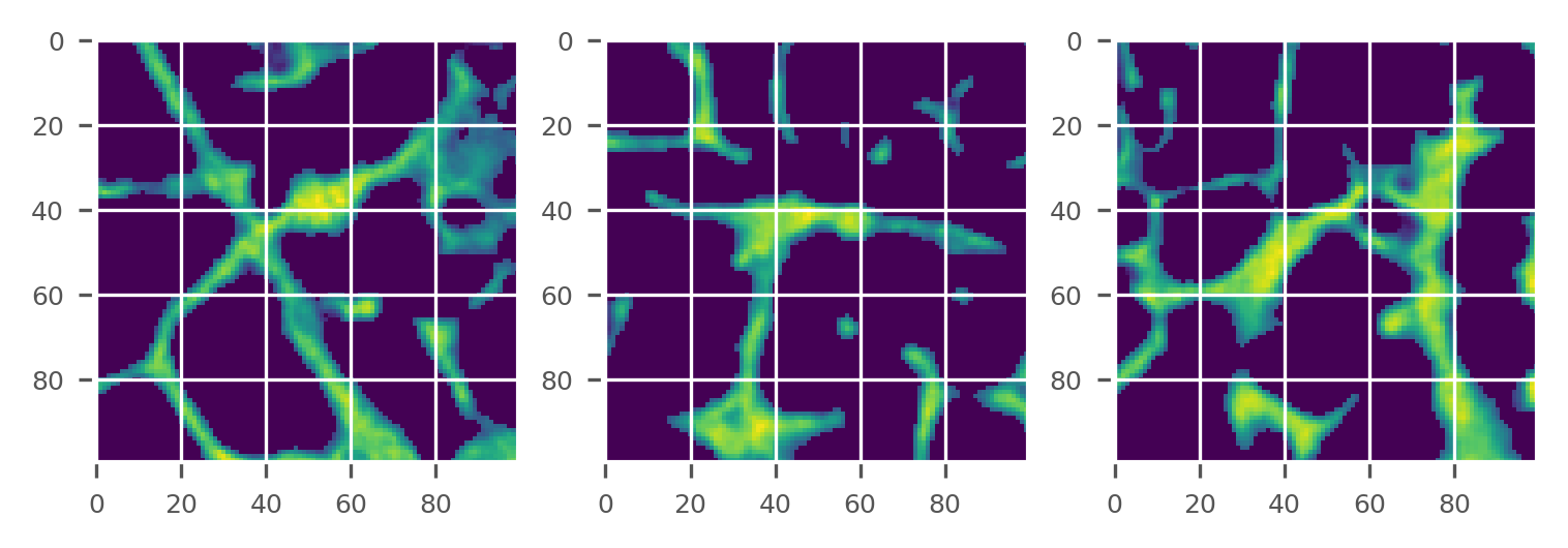
Mask the dataset
masked = data_3D.copy().astype('uint8')
masked[~L] = 0
plot_midplanes(masked)
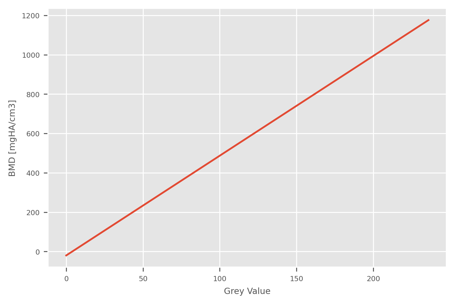
BMD calibration
Convert Hounsfield Units to Bone Mineral Density
BMD = HU*(slope_dens/muScaling) + offset_dens
slope_dens = 3650
muScaling = 720
offset_dens = -20

def HU2BMD(HU, slope_dens, muScaling, offset_dens):
    return HU*(slope_dens/muScaling) + offset_dens
Convert the masked 3D dataset
masked_BMD = HU2BMD(masked, slope_dens, muScaling, offset_dens)
Plot the HU->BMD calibration rule
fig, ax = plt.subplots()
plt.plot(np.unique(masked), HU2BMD(np.unique(masked), slope_dens, muScaling, offset_dens))
plt.xlabel('Grey Value')
plt.ylabel('BMD [mgHA/cm3]')
plt.show()
plt.style.use('ggplot')
Material mapping: BMD-Tissue modulus relationship [1, 2]
We convert local BMD values to Tissue Elastic Modulus applying the following law:
E_tissue = BMD * (E_ref/1.1e3) * b
Where E_ref is the compressive tissue modulus for fully mineralized (1100 mgHA/cm3) cortical bone (defined as 20 GPa), and b is an exponent defining the nature of the E-BMD relationship (i.e., b = 1 for a linear relationship).
b = 1
E_ref = 20000 # [MPa]
BMD_ref = 1.1e3 # [mgHA/cm3]

def BMD2E(BMD, E_ref=20e3, BMD_ref=1.1e3, b=1):
    return BMD*(E_ref/BMD_ref)*b
Plot the BMD->E calibration rule
fig, ax = plt.subplots()
plt.plot(np.unique(masked_BMD), BMD2E(np.unique(masked_BMD)))
plt.ylabel('Tissue Modulus [MPa]')
plt.xlabel('BMD [mgHA/cm3]')
plt.show()
plt.style.use('ggplot')

Convert the masked 3D dataset
masked_E = BMD2E(masked_BMD)
Cumulative Density Function of the Tissue Modulus
n_bins = 100
h, bins = np.histogram(masked_E[masked_E>0].ravel(), bins=n_bins)
Plot the resulting distribution of Tissue Modulus across the sample
fig, ax = plt.subplots()
ax1 = ax.twinx()
ax.hist(masked_E[masked_E>0].ravel(), bins=n_bins, alpha=0.4, density=True)
ax1.plot(bins[:-1], np.cumsum(h)/np.max(np.cumsum(h)))
ax.set_xlabel('Tissue elastic modulus [MPa]')
ax.set_ylabel('Counts')
ax1.set_ylabel('CDF')
plt.show()

Binning the heterogeneous Tissue Modulus image
Digitize the image based on the bins obtained above
masked_E_digitized = np.digitize(masked_E, bins, right=False)
Create list of binned Tissue Modulus values
E_digitized_values = (np.round((bins[1:]+bins[:-1])/2).tolist())
E_digitized_values.insert(0, 0)
E_digitized_values.append(np.round(bins[-1]))
Assign the digitized Tissue Modulus
for digit in np.unique(masked_E_digitized.ravel()):
    masked_E_digitized[masked_E_digitized==digit] = E_digitized_values[digit]
plot_midplanes(masked_E_digitized)

Generate Unstructured Grid Mesh of hexahedra from volume data
mesh = ciclope.core.voxelFE.vol2ugrid(masked_E_digitized, vs, verbose=True)
INFO:root:Calculating cell array
INFO:root:Detecting node coordinates and boundary nodes
INFO:root:Generated the following mesh with 1030301 nodes and 247058 elements:
INFO:root:<meshio mesh object>
  Number of points: 1030301
  Number of cells:
    hexahedron: 247058
  Point sets: NODES_Y1, NODES_Y0, NODES_X0, NODES_X1, NODES_Z1, NODES_Z0, NODES_X0Y0Z0, NODES_X0Y0Z1
  Cell sets: CELLS_Y1, CELLS_Y0, CELLS_X0, CELLS_X1, CELLS_Z1, CELLS_Z0
  Cell data: GV
print(mesh.cell_data)
{'GV': [array([ 5458, 7382, 11873, ..., 14867, 11445, 6313])]}
Write the mesh for checking using meshio
# filename_mesh_out = './../test_data/LHDL/3155_D_4_bc/results/3155_D_4_bc_voxelmesh.vtk'
# mesh.write(filename_mesh_out)
Write CalculiX input FE files
Generate voxel-FE model with heterogeneous material properties
If the input mesh contains field data GV, this can be mapped to heterogeneous material properties.artat=pt05ch17s02abm02.html
filename_out = './../../test_data/LHDL/3155_D_4_bc/results/3155_D_4_bc_matprop_voxelFE.inp'
input_template = "./../../input_templates/tmp_example01_comp_static_bone_matprop.inp"
Notice that this time we use an input template file which does not contain the material definition section.
!cat {input_template}
** ---------------------------------------------------
** Analysis definition. The Step module defines the analysis steps and associated output requests.
** More info at:
** https://abaqus-docs.mit.edu/2017/English/SIMACAECAERefMap/simacae-m-Sim-sb.htm#simacae-m-Sim-sb
** ---------------------------------------------------
*STEP
*STATIC
** All displacements fixed at bottom:
*BOUNDARY
NODES_Z0, 1, 3, 0.0
** Vertical displacement imposed at top:
*BOUNDARY
NODES_Z1, 3, 3, -0.04
** ---------------------------------------------------
** Output request:
*NODE FILE, OUTPUT=2D
U
*NODE PRINT, TOTALS=ONLY, NSET=NODES_Z0
RF
*EL FILE, OUTPUT=2D
S, E
*END STEP
Generate CalculiX input file with the voxelfe.mesh2voxelfe method. This time we activate the option matprop
help(ciclope.core.voxelFE.mesh2voxelfe)
Help on function mesh2voxelfe in module ciclope.core.voxelFE:

mesh2voxelfe(mesh, templatefile, fileout, matprop=None, keywords=['NSET', 'ELSET'], eltype='C3D8', matpropbits=8, refnode=None, verbose=False)
    Generate ABAQUS voxel Finite Element (FE) input file from 3D Unstructured Grid mesh data.
    The file written is an input file (.INP) in ABAQUS syntax that can be solved using ABAQUS or CALCULIX.
    The user can define a material mapping strategy for the conversion of local GVs to local material properties in the FE model.
    Material mapping laws are defined in separate template file(s) (see "prop.inp" and "property_temp_bone.inp" for examples).
    Boundary conditions, analysis type and output requests are defined in a separate template file (see "tmp.inp" for an example).
    Info on analysis definition at: https://abaqus-docs.mit.edu/2017/English/SIMACAECAERefMap/simacae-m-Sim-sb.htm#simacae-m-Sim-sb

    Parameters
    ----------
    mesh : meshio
        Unstructured grid mesh.
    templatefile : str
        Analysis template file.
    fileout : str
        Output .INP file.
    matprop : dict
        Dictionary of material properties for material property mapping:
        matprop = {
            "file": ["prop.inp", "property_temp_bone.inp", ...],
            "range": [[250, 255], [0, 250], ...],
        }
    keywords : str
        SUPPORTED ABAQUS KEYWORDS:

        For a list of all Abaqus keywords and their description visit:
        https://abaqus-docs.mit.edu/2017/English/SIMACAECAERefMap/simacae-c-gen-kwbrowser.htm#simacae-c-gen-kwbrowser__simacae-gen-xsl-U

        * 'NSET':
                Create boundary node sets. (Default = ON)
                If 'NSET' is specified, the following node sets are created:
                  - NODES_X0: Nodes on WEST (X-) surface of 3D model.
                  - NODES_X1: Nodes on EAST (X+) surface of 3D model.
                  - NODES_Y0: Nodes on SOUTH (Y-) surface of 3D model.
                  - NODES_Y1: Nodes on NORTH (Y+) surface of 3D model.
                  - NODES_Z0: Nodes on BOTTOM (Z-) surface of 3D model.
                  - NODES_Z1: Nodes on TOP (Z+) surface of 3D model.
                  - NODES_X0Y0Z0: 2 nodes on (0,0,0) model corner.
                  - NODES_X0Y0Z1: 2 nodes on (0,0,1) model corner.
                These node sets are available for boundary conditions definition.
        * 'ELSET':
                Create boundary element sets. (Default = ON)
                If 'ELSET' is specified, the following element sets are created:
                  - ELEMS_X0: Elements of WEST (X-) surface of 3D model.
                  - ELEMS_X1: Elements of EAST (X+) surface of 3D model.
                  - ELEMS_Y0: Elements of SOUTH (Y-) surface of 3D model.
                  - ELEMS_Y1: Elements of NORTH (Y+) surface of 3D model.
                  - ELEMS_Z0: Elements of BOTTOM (Z-) surface of 3D model.
                  - ELEMS_Z1: Elements of TOP (Z+) surface of 3D model.
        * 'PROPERTY':
                Define an external material mapping law from template file. (Default = None)
                Use in combination with 'matprop' dictionary of material property files and corresponding GV ranges for the material mapping.
    eltype : str
        FE element type. The default is eight-node brick element (C3D8 and F3D8). See CalculiX node convention (Par. 6.2.1) at: http://www.dhondt.de/ccx_2.15.pdf
    matpropbits : int
        Bit depth for material mapping.
    refnode
        Reference node coordinates [REF_NODE_x, REF_NODE_y, REF_NODE_z] for kinematic coupling.
    verbose : bool
        Activate verbose output.
ciclope.core.voxelFE.mesh2voxelfe(mesh, input_template, filename_out, verbose=True,
                             keywords=['NSET', 'ELSET', 'PROPERTY'],
                             matprop = {
                                 "file": ["./../../material_properties/bone_Etissue.inp"],
                                 "range": [[1, 22000]]
                                       },
                             matpropbits=16)
INFO:root:Found cell_data: GV. cell_data range: 112 - 21389.
INFO:root:Checking GV range for user material properties
INFO:root:Start writing INP file
INFO:root:Writing model nodes to INP file
INFO:root:Writing model elements to INP file
INFO:root:Additional nodes sets generated: ['NODES_Y1', 'NODES_Y0', 'NODES_X0', 'NODES_X1', 'NODES_Z1', 'NODES_Z0', 'NODES_X0Y0Z0', 'NODES_X0Y0Z1']
INFO:root:Additional cell sets generated: ['CELLS_Y1', 'CELLS_Y0', 'CELLS_X0', 'CELLS_X1', 'CELLS_Z1', 'CELLS_Z0']
INFO:root:User material properties defined. Writing material property section of INP file
INFO:root:Reading Abaqus template file ./../../input_templates/tmp_example01_comp_static_bone_matprop.inp
INFO:root:Model with 1030301 nodes and 247058 elements written to file ./../../test_data/LHDL/3155_D_4_bc/results/3155_D_4_bc_matprop_voxelFE.inp
Run in CalculiX
!export OMP_NUM_THREADS=8; ccx_2.17_MT "./../../test_data/LHDL/3155_D_4_bc/results/3155_D_4_bc_matprop_voxelFE"
************************************************************

CalculiX Version 2.17, Copyright(C) 1998-2020 Guido Dhondt
CalculiX comes with ABSOLUTELY NO WARRANTY. This is free
software, and you are welcome to redistribute it under
certain conditions, see gpl.htm

************************************************************

You are using an executable made on Sun 10 Jan 2021 11:34:19 AM CET

  The numbers below are estimated upper bounds

  number of:

   nodes:      1030289
   elements:       247058
   one-dimensional elements:            0
   two-dimensional elements:            0
   integration points per element:            8
   degrees of freedom per node:            3
   layers per element:            1

   distributed facial loads:            0
   distributed volumetric loads:            0
   concentrated loads:            0
   single point constraints:        11787
   multiple point constraints:            1
   terms in all multiple point constraints:            1
   tie constraints:            0
   dependent nodes tied by cyclic constraints:            0
   dependent nodes in pre-tension constraints:            0

   sets:          115
   terms in all sets:       287847

   materials:          101
   constants per material and temperature:            2
   temperature points per material:            1
   plastic data points per material:            0

   orientations:            0
   amplitudes:            2
   data points in all amplitudes:            2
   print requests:            1
   transformations:            0
   property cards:            0


 STEP            1

 Static analysis was selected

 Decascading the MPC's

 Determining the structure of the matrix:
 number of equations
 997038
 number of nonzero lower triangular matrix elements
 32629475

 Using up to 8 cpu(s) for the stress calculation.

 Using up to 8 cpu(s) for the symmetric stiffness/mass contributions.

 Factoring the system of equations using the symmetric spooles solver
 Using up to 8 cpu(s) for spooles.

 Using up to 8 cpu(s) for the stress calculation.


 Job finished

________________________________________

Total CalculiX Time: 236.322873
________________________________________
Post-processing of FE results
Convert Calculix output to Paraview
filename_out_base, ext_out = os.path.splitext(filename_out)
ccx2paraview.Converter(filename_out_base + '.frd', ['vtk']).run()
INFO:root:Reading 3155_D_4_bc_matprop_voxelFE.frd
INFO:root:336275 nodes
INFO:root:247058 cells
INFO:root:Step 1, time 1.0, U, 3 components, 336275 values
INFO:root:Step 1, time 1.0, S, 6 components, 336275 values
INFO:root:Step 1, time 1.0, E, 6 components, 336275 values
INFO:root:Step 1, time 1.0, ERROR, 1 components, 336275 values
INFO:root:1 time increment
INFO:root:Writing 3155_D_4_bc_matprop_voxelFE.vtk
INFO:root:Step 1, time 1.0, U, 3 components, 336275 values
INFO:root:Step 1, time 1.0, S, 6 components, 336275 values
INFO:root:Step 1, time 1.0, S_Mises, 1 components, 336275 values
INFO:root:Step 1, time 1.0, S_Principal, 3 components, 336275 values
INFO:root:Step 1, time 1.0, E, 6 components, 336275 values
INFO:root:Step 1, time 1.0, E_Mises, 1 components, 336275 values
INFO:root:Step 1, time 1.0, E_Principal, 3 components, 336275 values
INFO:root:Step 1, time 1.0, ERROR, 1 components, 336275 values
Reaction forces
!cat {filename_out_base+'.dat'}
 total force (fx,fy,fz) for set NODES_Z0 and time  0.1000000E+01

        1.131664E-13 -2.036052E-12  1.370934E+02
Apparent elastic modulus
E_app = (F_tot / A) / epsilon
A = 200*0.0195*200*0.0195 # [mm2]
epsilon = 0.04/(200*0.0195)
E = (1.37e2/A)/epsilon
print(f"{E:.2f} MPa")
878.21 MPa
Bone volume fraction
BVTV = 100*np.sum(L)/L.size
print(f"{BVTV:.2f} %")
24.71 %
Visualize results in Paraview
!paraview {filename_out_base + '.vtk'}

Dependencies
import watermark
%load_ext watermark

%watermark
%watermark --iversions
Last updated: 2023-01-20T22:37:51.286853+03:00

Python implementation: CPython
Python version       : 3.8.15
IPython version      : 8.8.0

Compiler    : GCC 10.4.0
OS          : Linux
Release     : 4.19.0-23-amd64
Machine     : x86_64
Processor   :
CPU cores   : 8
Architecture: 64bit

watermark : 2.3.1
sys       : 3.8.15 | packaged by conda-forge | (default, Nov 22 2022, 08:49:35)
[GCC 10.4.0]
ciclope   : 1.3.0
dxchange  : 0.0.1
scipy     : 1.8.1
skimage   : 0.18.1
matplotlib: 3.5.2
numpy     : 1.24.1
References
Bourne, Benjamin C., and Marjolein C. H. van der Meulen. 2004. “Finite Element Models Predict Cancellous Apparent Modulus When Tissue Modulus Is Scaled from Specimen CT-Attenuation.” Journal of Biomechanics 37 (5): 613–21. https://doi.org/10.1016/j.jbiomech.2003.10.002.
Cox, Jason M., Joshua D. Smith, Marjolein C. H. van der Meulen, and Jacqueline H. Cole. 2022. “Heterogeneous Tissue Modulus Improved Prediction of Mechanical Behavior in Osteoporotic Vertebral Cancellous Bone.” bioRxiv. https://doi.org/10.1101/2021.11.30.470675.
Acknowledgements
This notebook was developed within Building the Jupyter Community in MSK Imaging Research, a Jupyter Community Workshop sponsored by NUMFocus